Hydraulic Modeling of Complex Fluids
Hydraulic Modeling of Complex Fluids
Keywords
Share
Summary
Modeling of complex fluids like non-Newtonian fluids or settling slurries should not be intimidating. The basic steps are very similar to that of conventional hydraulic models for single-phase, Newtonian fluids like water.
However, a few additional set-up steps are required as you build your model. Fathom and Impulse both have the capabilities of modeling non-Newtonian fluids built-in to the traditional software package. But to model settling slurries, the Settling Slurry add-on module is required. Once again, both Fathom and Impulse have the option to add this module. This file will go over the basic information and steps required to model these types of fluids. This file will not delve deep into the theory behind the fluid dynamic principles, but rather focus on the process of building a hydraulic model. It is essential to have a good understanding of fluid dynamic principles utilized in this topic.
Non-Newtonian fluids are fluids whose viscosity changes as shear force, τ, is applied on the fluid. This change in viscosity can be characterized by different models and it makes their behavior harder to model. Some of the different classifications and behaviors of non-Newtonian fluids are seen in Figure 1.
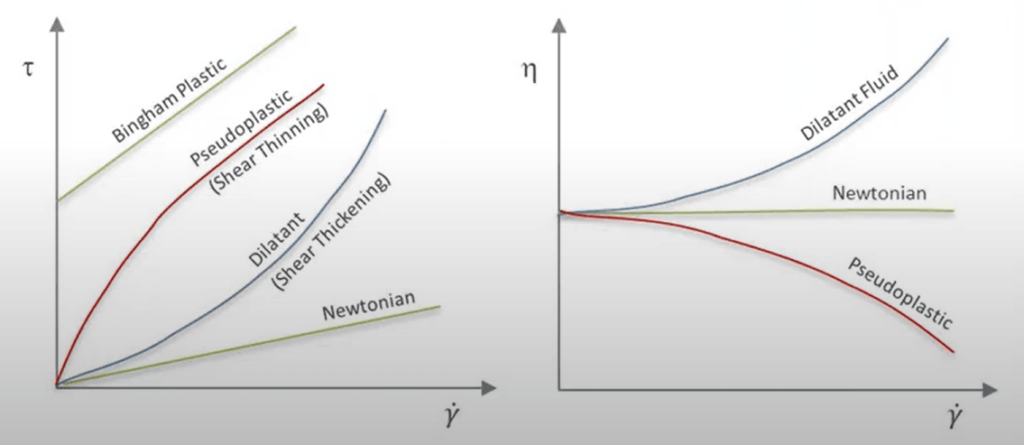
Figure 1: Non-Newtonian fluids behavior and classification
Slurries are mixtures of solids suspended in a liquid, usually water. Slurries can sometimes be modelled as regular fluids with appropriate specific gravity and viscosities. However, based on their rheology and compositions, they may sometimes behave as non-Newtonian fluids. Additionally, slurries can be characterized as settling or non-settling. Non-settling slurries behave as a homogeneous mixture with solids suspended evenly. Settling slurries behave as heterogenous mixtures where flow velocity can affect solid particle suspension. Aside from the need to calculate a minimum flow velocity to maintain solid suspension (settling velocity), this solid-fluid interaction can cause settling slurries to behave in a more complex manner and affect the following fluid characteristics:
- System curve
- Viscosity
- Specific gravity
- Hydraulic gradient
Codes and Standards
Solution/Best Practice
The first step and most difficult step in dealing with complex fluids is to obtain rheology data for the fluid.
This is typically obtained through laboratory studies of the fluid in question. Rheology data typically contains the following parameters:
- Tabulated viscosity data (shear stress vs shear rate; viscosity vs RPM of test equipment; viscosity vs shear rate; viscosity vs velocity) or viscosity model constants
- Specific gravity
- Chemical composition
- Solids composition data: percentage of solids, particle size and distribution
Most non-Newtonian fluids and slurries that are encountered in project work will be specific mixtures or solutions created by the specific process conditions encountered, and thus will have different characteristics every time. Typically, there will not be published rheology data readily available nor a practical way to predict the fluids properties. On most applications, rheology data will need to be requested from the client or a rheology study will need to be conducted to determine the fluid properties and stablish a viscosity model. The options available to the designer to determine the appropriate fluid properties required to build the hydraulic model are as follows:
- Request the applicable rheology data for the application from the client as they may have reported rheology for the process.
- Conduct a laboratory rheology study to obtain a complete report outlining all applicable fluid properties and viscosity model parameters. These studies can utilize different styles or rheometers to characterize the fluid properties.
- Conduct field measurements to obtain the desired data to complete the model within the operating range of the system. This can be as simple as capturing pressure drop vs velocity data. Note that this may not be as thorough or accurate as a full laboratory study.
- Search for any published models or research on similar fluids or applications. Fluids with more common chemical compositions may have already been studied in detail and the desired data may be readily available.
- Contact to pump manufacturers (specifically those already in use by the client) as they may have experience or data for the system in question or similar applications. Some pump manufacturers have published viscosity for models for common applications.
For Non-Newtonian fluids, the main design parameter required for the hydraulic model will be the tabulated viscosity data or the applicable viscosity model. Viscosity models provide a method to predict the fluid’s viscosity at different conditions. Fathom has built in tools to enter the paraments related to each viscosity model. A thorough rheology study will outline what viscosity model can be used to represent the fluid, and the parameters that govern that model’s relation. These parameters will be required to model the fluid in Fathom. While using the software, the viscosity model can be selected on the “System Properties” input window, under the “Viscosity Model” tab. Some of the most common viscosity models are as follows:
- Bingham Plastics: Used to capture fluids with a yield stress (yield stress required for fluid to flow). The apparent viscosity is dependent on the yield stress (Sy) and the coefficient of rigidity (Rc), which are the parameters you will need to enter in Fathom as seen in Figure 2. These can also be calculated from rheological data. It is important to note that since Bingham plastics require a minimum yield stress to flow, fathom may not be able to generate a system curve at low flows. Fathom would run into an error if this were the case, and a minimum flow will need to be specified to generate the system curve.

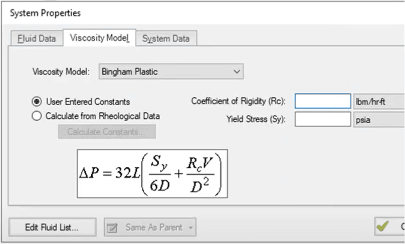
Figure 2: Bingham Plastic model Fathom input window.
Power Law Fluid: Common model broadly used in industry. This model relies on power law correlations for shear stress and apparent viscosity. These correlations contain the parameters K (flow consistency index) and n (flow behavior index) which will need to be input into Fathom as seen on Figure 3. These can also be calculated from rheological data.

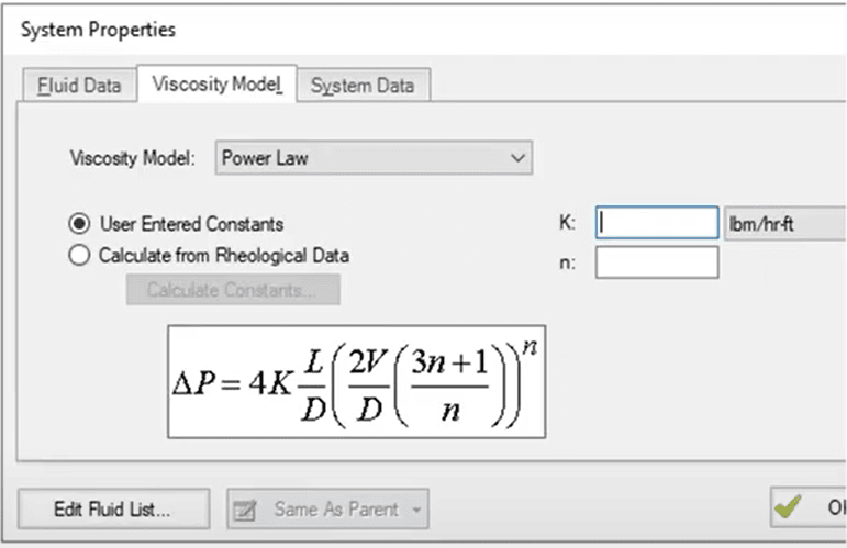
Figure 3: Power Law model Fathom input window.
Homogeneous Scale-Up Model:Broadest model type that can be used to capture any fluid type. Relies on test data for pressure loss vs. velocity, which is entered into Fathom as seen on Figure 4. Test data is then scaled up to the system based on the pipe diameter used in the model.
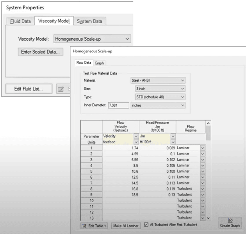
Figure 4: Homogeneous scale-up model Fathom input window.
Paper Stock – Duffy Model: General model for pump stocks in pipes. User selects pulp type and consistency, and system determines head loss based on velocity correlations from the Technical Association from the Pulp and Paper Stock Industry. The Fathom input window and required data can be seen in Figure 5.
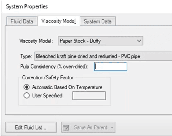
Figure 5: Homogeneous scale-up model Fathom input window.
Paper Stock – Brecht and Heller: A more conservative model for pulp stocks in pipes. User selects pulp type and consistency, and system determines head loss from correlations based on Reynolds number and friction factor. The Fathom input window and required data can be seen in Figure 6.
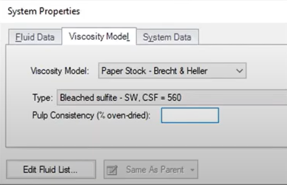
Figure 6: Paper stock Brecht & Heller model Fathom input window
Once the appropriate Viscosity model is selected, and the required parameters provided, the rest of the process will be the same as modeling a simple Newtonian fluid, including your output window and results. However, users can run different conditions (pump speed, available head, different flow rates) to see how the viscosity changes based on different conditions and what effects it has on your system capacity and system curve.
Modeling slurries will add another layer of complexity to your Fathom model. Aside from choosing the right viscosity model for your slurry (often slurries will behave as a Bingham plastic), settling information may also be considered. Fathom has an add-on module for settling slurries, which allows input of detailed slurry properties. Some slurries are dilute enough to that they can be modeled as a regular Newtonian fluid with appropriate viscosity and density. But with heavier concentration slurries, solids composition starts to play a bigger effect in the behavior of the fluid. The inclusion of solids composition data into the model will allow result in a more accurate system curve and to ensure no settling of solids occurs in the system. In fathom, once the settling slurry module is turned on, the “System Properties” input window now offer the following inputs:
- Basic Water Slurry Input: Options for minimal, simplified, and detailed models. The detailed model will require the following properties:
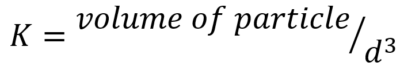
- Terminal Velocity Parameter: Shape Factor (K) or the parameter ξ, which is the ratio Vt/Vts, where Vt is terminal settling velocity of a non-spherical particle and Vts the terminal velocity of a spherical particle with the same diameter. The shape factor K may be found from the equation below. This data will either be obtained from rheological studies, or from researching tabulated/published for the minerals present in the slurry.
- Particle side distribution (d50 and d85): Refers to measure of the percentage of particles in the slurry with a certain size of smaller. A slurry with a d85 of 3mm means that 85% of the particles have a diameter of 3mm or less. This data will come from rheological studies or from process design parameters (expected performance of grinding circuit, cyclones, filters, etc.).
- Fluid Temperature
- Solids concentration, option for volume fraction, mass fraction, or solids ratio.
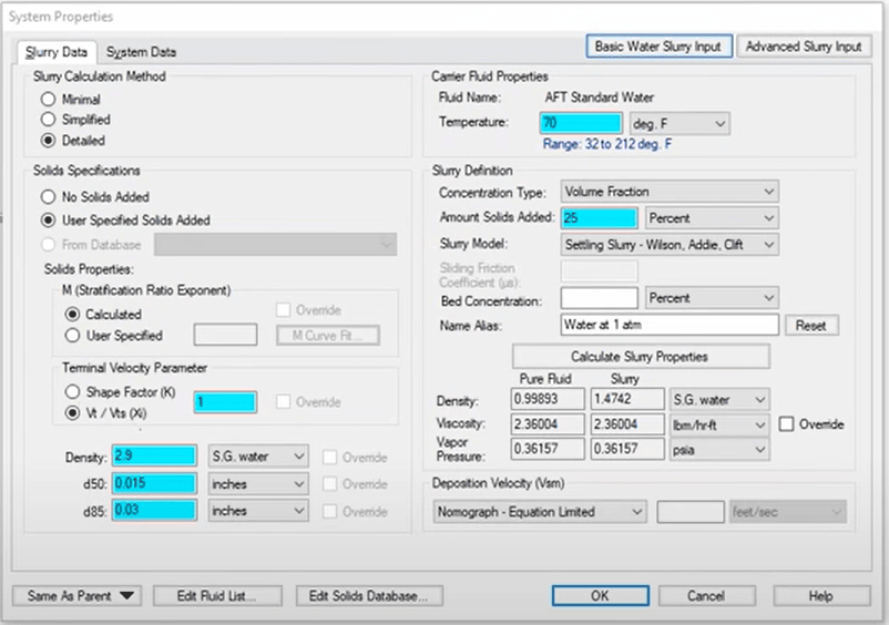
Figure 7: System properties input widow with settling slurry module enabled.
- Advanced Slurry Input: Allows you to define more complex slurries with carrier fluid other than water.
System curves for pumps are given for water. Correction factors must pe specified to de-rate the pump performance based on the specific slurry. Fathom allows you to account for this based on a few different methods as seen in Figure 8. In the example below, you need to enter the percentage of fine particles for the slurry and the pump impeller size.
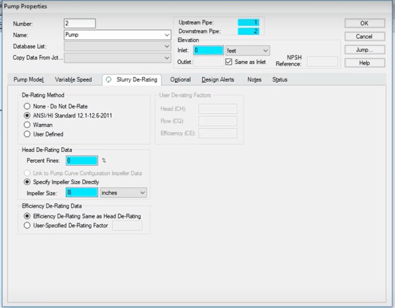
Figure 8: Pump properties slurry de-rating input window.
The settling slurries add-on module will include additional functionality for the outputs and results windows. Fathom will now display a slurry tab as seen in Figure 9, which can include hydraulic gradients (Im & Jm), settling velocity, slurry head, and mass flow rate of mixture, liquid, and solids. More parameters are available on the “Output Control” window to gain a comprehensive understanding of the slurry behavior and aid in the design of the system. The “Pump Summary” tab will now display information about the correction factors required for flow, head and efficiency which will be needed to specify the appropriate pump and motor. Additionally, the “Graph Results” tab will have the ability to plot slurry specific results such as slurry system curve, and mixture hydraulic gradient (Jm). All of these are power tools to aid in the design of slurry systems.
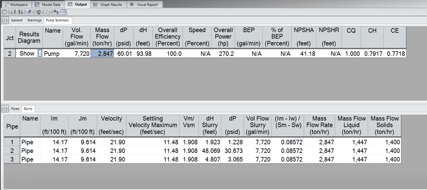
Figure 9: Settling slurry output window.
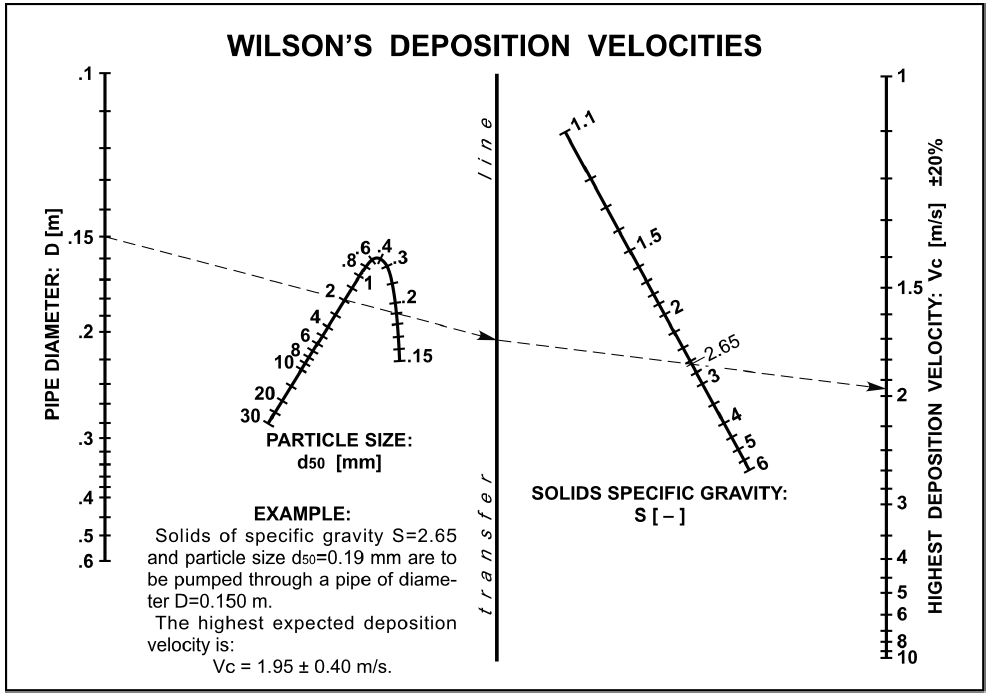
In the absence of the settling slurry addon module on Fathom, a simplified hydraulic model of the slurry could be created by simply accounting for the appropriate viscosity model and density. The settling velocity then may be calculated by hand with the use of nomographic charts depicted in Figures 10 and 11. These monograms are commonly used in industry for simpler slurries and will provide a conservative estimation of the settling velocities. This can the be used to check your line size with your hydraulic model to ensure none of the lines in the system go below this velocity threshold. It should be noted that these monograms have limitations and will not be as accurate as the built-in empirical calculations in Fathom, specially with slurries with a more complex composition and particle distribution. Another limitation of this approach of modeling a slurry is a reduced accuracy in hydraulic gradient calculations, as the behavior of the solids in the mixture would not be considered. This approach should not be relied on if solids concentration Cv > 50%.
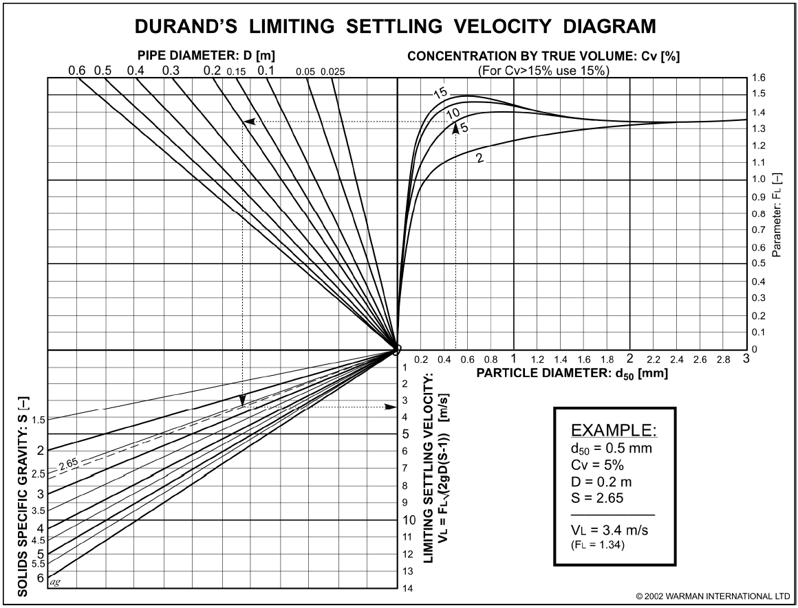
Figure 10: Durand’s nomogram for calculating settling velocity.